Source Terms
Introduction
Source terms are additional physics that appear on the right-hand side of the fluid equations, modifying the conserved variables without changing the underlying Godunov update. AthenaK applies them at every stage of the Runge–Kutta integrator, after the flux divergence has been computed. Typical examples are an external gravitational acceleration, optically thin radiative cooling, and a rotating-frame (shearing-box) force.
Source terms are configured in blocks that are separate from the physics blocks: hydro
source terms go in <hydro_srcterms>, MHD source terms in <mhd_srcterms>, and radiation
source terms in <rad_srcterms>. Simply adding the relevant block (with a term enabled)
turns the physics on. Random turbulent forcing is handled by a dedicated driver and is
configured in its own <turb_driving> block; the shearing box is documented separately (see
Shearing Box).
Inputs
Constant acceleration
A spatially uniform acceleration (e.g. an external gravity field), configured in
<hydro_srcterms> or <mhd_srcterms>:
const_accel(defaultfalse): enable the term.const_accel_val(mandatory if enabled): the acceleration \(g\).const_accel_dir(mandatory if enabled): direction,1,2, or3for the x1/x2/x3 momentum component.
Optically thin cooling
ISM cooling (with a SPEX-based cooling curve) plus uniform heating:
ism_cooling(defaultfalse): enable ISM cooling/heating.hrate(mandatory if enabled): uniform heating rate. Requires a<units>block for the CGS conversion (see Units).
A relativistic optically thin cooling term is also available:
rel_cooling(defaultfalse): enable relativistic cooling (acts on energy and momentum).crate_rel(mandatory if enabled): cooling-rate coefficient.cpower_rel(default1.0): power-law exponent applied to \((T\,\text{crate\_rel})\).
Both cooling terms impose their own cooling-limited timestep.
Radiation beam
Configured in <rad_srcterms> to inject a collimated beam of radiation (see
Radiation): rad_beam, dii_dt, pos_1/2/3, dir_1/2/3, width, and
spread (beam opening angle in degrees).
Turbulent driving
Solenoidal Ornstein–Uhlenbeck forcing in a periodic box, configured in <turb_driving>:
dedt(default0): target energy-injection rate.tcorr(default0): correlation time of the forcing (\(\lesssim 10^{-6}\) gives white-in-time noise).nlow(default1) /nhigh(default2): range of integer wavenumbers driven.driving_type(default0):0isotropic (usesexpo),1anisotropic (usesexp_prpandexp_prl).expo(default5/3): power-law exponent of the driving spectrum for isotropic driving.
User source terms
Setting <problem>/user_srcs = true calls a user-supplied function (registered by a custom
problem generator) each stage, allowing arbitrary problem-specific source terms.
Outputs
Source terms do not add their own output fields — they modify the standard fluid variables, so
you visualize their effect through the usual hydro_w / mhd_w_bcc outputs (see
Hydrodynamics, Magnetohydrodynamics, and Outputs). The one exception is turbulent driving, whose force
field can be dumped with variable = turb_force (components force1, force2,
force3).
Example: gravity-driven Rayleigh–Taylor instability
The Rayleigh–Taylor instability (RTI) places a dense fluid on top of a lighter one in a
constant gravitational field — a direct application of the constant-acceleration source term.
AthenaK ships an input file at inputs/hydro/rt2d.athinput.
1. Build the RT problem generator (this is a custom problem generator, selected at build time):
cmake -B build -DPROBLEM=rt
cmake --build build -j
2. Inspect the source term. In inputs/hydro/rt2d.athinput the gravity is switched on
in the <hydro_srcterms> block:
<hydro_srcterms>
const_accel     = true   # add constant acceleration source term
const_accel_val = -0.1   # value of the acceleration g
const_accel_dir = 2      # apply it along x2 (vertical)
3. Slightly modify it. Switch the output to the native binary format and, for a livelier
image, use the multimode initial perturbation by editing <problem>:
<problem>
iprob = 2       # 2 = random (multimode) perturbations
amp   = 0.05
drat  = 3.0
smooth_interface = true

<output2>
file_type  = bin       # native binary dump
variable   = hydro_w
dt         = 0.1
4. Run and visualize:
./build/src/athena -i inputs/hydro/rt2d.athinput -d run
python3 vis/python/plot_slice.py run/bin/RTI.out2.00030.bin dens rt_dens.png
The dense fluid sinks in narrow spikes while the light fluid rises in broad bubbles:
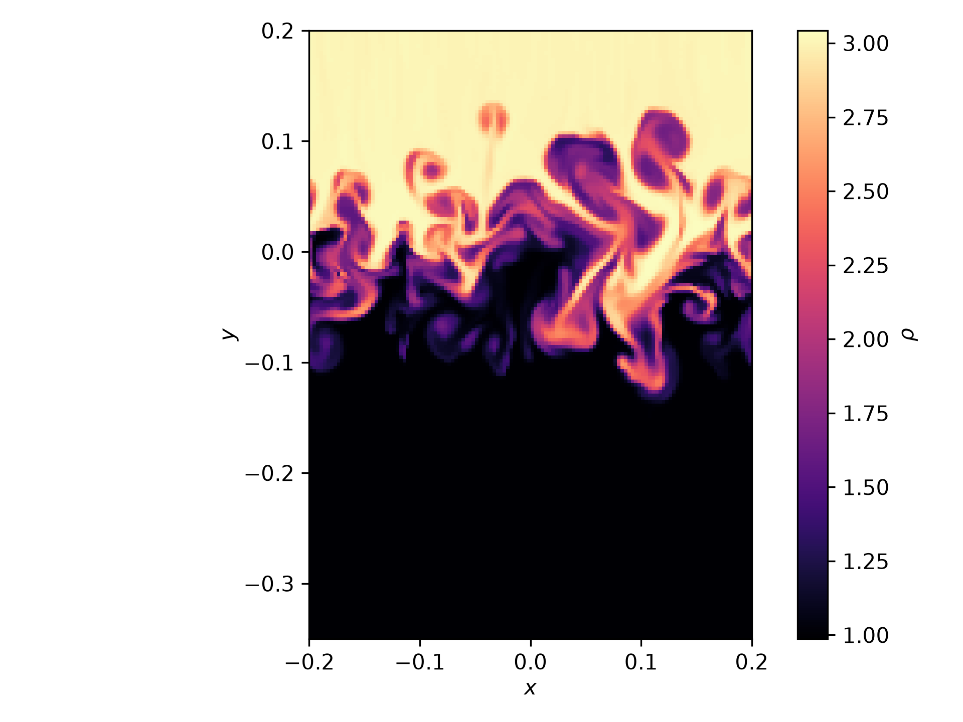
Increasing const_accel_val (stronger gravity) makes the instability grow faster; note
that the RT problem generator reads the same acceleration from the <hydro> block to set up
the initial hydrostatic pressure, so keep the two values consistent if you change it.