Magnetohydrodynamics

Introduction

The MHD solver extends the hydrodynamics module to magnetized flows. It uses the same reconstruct–solve–update Godunov machinery for the gas variables, and additionally evolves the magnetic field with constrained transport (CT), which keeps the discrete divergence of the field at machine precision. Like the hydro solver it supports Newtonian, special relativistic, and general relativistic regimes, selected through the coordinate system and equation of state.

MHD is enabled by including an <mhd> block in the input file.

Note

A single run may not contain both <hydro> and <mhd> unless it is a two-fluid ion–neutral calculation (see Ion-Neutral Fluids).

Inputs

The <mhd> block shares most of its parameters with <hydro>:

• eos (mandatory): ideal or isothermal.

• gamma / iso_sound_speed: as for hydro (one is mandatory depending on eos).

• reconstruct (default plm): dc, plm, ppm4, ppmx, or wenoz (the higher-order options require more ghost zones).

• rsolver (mandatory): approximate Riemann solver. Valid choices:

  • Newtonian MHD: llf, hlle, hlld

  • special/general relativistic MHD: llf, hlle

  • kinematic evolution: advect

• nscalars (default 0): number of passive scalars.

• fofc (default false): first-order flux correction.

• floors/ceilings: dfloor, pfloor, tfloor, sfloor, gamma_max (SR/GR).

MHD-specific options:

• sigma_max (SR/GR): magnetization ceiling \(\sigma = b^2/(\rho h)\) used in the conserved-to-primitive floors.

• ohmic_resistivity: if present, enables Ohmic resistivity with the given coefficient (see Explicit Diffusion).

The initial magnetic field itself is set by the problem generator. Source terms live in the separate <mhd_srcterms> block (see Source Terms).

Outputs

Request one of the following in an <output>/variable line (see Outputs):

• mhd_w: all primitive gas variables.

• mhd_u: all conserved gas variables.

• mhd_bcc: the cell-centered magnetic field (bcc1, bcc2, bcc3).

• mhd_w_bcc / mhd_u_bcc: primitives / conserved variables with the cell-centered field appended.

Individual components (mhd_w_d, mhd_bcc1, …) and derived diagnostics are also available, including current density (mhd_jz, mhd_j2) and the discrete field divergence (mhd_divb), which is a useful check on the constrained-transport scheme.

Example: the Orszag–Tang vortex

The Orszag–Tang vortex is a classic 2D MHD test that develops into supersonic MHD turbulence, making it a good showcase for the MHD solver. AthenaK ships an input file at inputs/mhd/orszag_tang.athinput using the built-in orszag_tang problem generator.

1. Build (the orszag_tang generator is built in, so the default build suffices):

cmake -B build
cmake --build build -j

2. Slightly modify the input file. Starting from inputs/mhd/orszag_tang.athinput, drop the resolution a bit so it runs quickly (set the <mesh> and <meshblock> sizes to 256) and switch the field output from legacy VTK to the native binary format:

<output2>
file_type  = bin        # native binary dump
variable   = mhd_w_bcc  # primitives + cell-centered B
dt         = 0.05

3. Run:

./build/src/athena -i inputs/mhd/orszag_tang.athinput -d run

AthenaK names binary dumps <basename>.<variable>.<number>.bin. With dt = 0.05 the dump at \(t = 0.5\) is number 00010.

4. Visualize. For a quick look at a single field, the bundled slice plotter takes a .bin dump, a variable name, and an output image (the --notex flag avoids requiring a LaTeX install for the labels):

python3 vis/python/plot_slice.py run/bin/OrszagTang.mhd_w_bcc.00010.bin eint eint.png --notex

Derived quantities such as the magnetic energy \(B^2\) are easy to build from the cell-centered field stored in the mhd_w_bcc dump using the bundled reader vis/python/bin_convert.py (run the snippet from vis/python/ or add it to your PYTHONPATH):

import numpy as np
import matplotlib.pyplot as plt
from bin_convert import read_binary

d = read_binary("run/bin/OrszagTang.mhd_w_bcc.00010.bin")
nx1, nx2 = d["nx1_mb"], d["nx2_mb"]

def stitch(field):  # assemble MeshBlocks onto the (uniform) root grid
    out = np.zeros((d["Nx2"], d["Nx1"]))
    for m in range(d["n_mbs"]):
        i, j = d["mb_logical"][m][0], d["mb_logical"][m][1]
        out[j*nx2:(j+1)*nx2, i*nx1:(i+1)*nx1] = field(m)
    return out

eint = stitch(lambda m: d["mb_data"]["eint"][m][0])
b2 = stitch(lambda m: d["mb_data"]["bcc1"][m][0]**2
                       + d["mb_data"]["bcc2"][m][0]**2
                       + d["mb_data"]["bcc3"][m][0]**2)

ext = [d["x1min"], d["x1max"], d["x2min"], d["x2max"]]
fig, axs = plt.subplots(1, 2, figsize=(9.4, 4.3))
for ax, data, cmap, lab in [(axs[0], eint, "viridis", "internal energy $e$"),
                            (axs[1], b2, "inferno", "$B^2$")]:
    im = ax.imshow(data, origin="lower", extent=ext, cmap=cmap)
    ax.set_xlabel("x"); ax.set_ylabel("y"); ax.set_aspect("equal"); ax.set_title(lab)
    fig.colorbar(im, ax=ax, fraction=0.046, pad=0.04)
fig.suptitle("Orszag-Tang vortex at t = {:.1f}".format(d["time"]))
fig.tight_layout(); fig.savefig("orszag_tang.png", dpi=150)

The internal energy and magnetic energy at \(t = 0.5\) already show the sharp shocks and current sheets that make this such a demanding test:

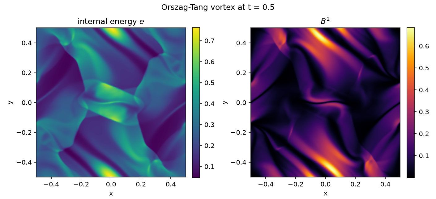
Try re-running with reconstruct = wenoz (and <mesh>/nghost = 4) or a finer grid to see how the small-scale current sheets sharpen.