Explicit Diffusion

Introduction

Alongside the ideal (non-dissipative) solvers, AthenaK can add explicit diffusion terms to the fluid and induction equations:

• Viscosity — diffusion of momentum (shear and, optionally, anisotropic viscosity).

• Thermal conduction — diffusion of heat (isotropic, anisotropic, or Spitzer).

• Resistivity — diffusion of the magnetic field (Ohmic and ambipolar).

Each process is implemented as an additional flux that is added to the face-centered fluxes of the conserved variables every stage of the Runge–Kutta integrator. Because the terms are treated explicitly, they impose a diffusive stability limit on the time step,

\[\Delta t \lesssim \frac{(\Delta x)^2}{D},\]

where \(D\) is the relevant diffusivity. For strongly diffusive problems this can dominate the cost, and the ideal (advective) CFL condition no longer sets the step.

Viscosity and thermal conduction can be added to either the <hydro> or the <mhd> block; resistivity is only meaningful for MHD and lives in the <mhd> block.

Inputs

Viscosity (in <hydro> or <mhd>):

• nu_iso (default 0): coefficient of isotropic (kinematic) shear viscosity \(\nu\).

• nu_aniso (default 0): coefficient of anisotropic (Braginskii) viscosity.

The isotropic viscous stress diffuses momentum, with a heating term added to the energy equation so that total energy is conserved.

Thermal conduction (in <hydro> or <mhd>):

• alpha_iso (default 0): coefficient of isotropic thermal diffusivity \(\alpha\).

• alpha_aniso (default 0): coefficient of anisotropic (field-aligned) thermal diffusivity.

• alpha_spitzer (default false): use a temperature-dependent Spitzer conductivity rather than a constant coefficient.

• q_limit: cap on the heat flux magnitude (saturated conduction); unlimited by default.

Note

The conduction coefficients alpha_* are diffusivities, not conductivities. The conductivity is \(\kappa = \rho\,\alpha\) and the heat flux is \(\boldsymbol{Q} = -\kappa\,\nabla T = -\rho\,\alpha\,\nabla T\). AthenaK uses a dimensionless temperature \(T = P/\rho\) (the factor \(\bar{m}/k_{\rm B}\) is not included), so alpha_iso must be given in the corresponding dimensionless units (see Units).

Resistivity (in <mhd>):

• eta_ohm (default 0): Ohmic resistivity \(\eta_{\rm O}\).

• eta_ad (default 0): ambipolar diffusivity \(\eta_{\rm A}\) (the effective diffusivity \(\eta_{\rm O} + \eta_{\rm A} B^2\) then varies in space).

A process is active whenever its coefficient is non-zero; for example, adding

<mhd>
nu_iso    = 1.0e-3   # shear viscosity
alpha_iso = 1.0e-3   # thermal diffusivity
eta_ohm   = 1.0e-2   # Ohmic resistivity

enables viscosity, conduction, and Ohmic resistivity together in an MHD run.

Governing equations

The dissipative fluxes added to the conserved-variable equations are

\[\Pi_{ij} = \rho\,\nu\left(\partial_i v_j + \partial_j v_i - \tfrac{2}{3}\,\delta_{ij}\nabla\!\cdot\!\boldsymbol{v}\right), \qquad \boldsymbol{Q} = -\rho\,\alpha\,\nabla T, \qquad \boldsymbol{\mathcal{E}}_{\rm O} = \eta_{\rm O}\,\nabla\times\boldsymbol{B},\]

for the viscous stress, heat flux, and Ohmic electric field respectively. Each reduces, for a small perturbation on a uniform background, to a simple diffusion equation \(\partial_t q = D\,\nabla^2 q\) for the diffusing quantity \(q\) (a velocity component, the temperature, or a magnetic-field component), with diffusivity \(D\) equal to \(\nu\), \((\gamma-1)\,\alpha\), and \(\eta_{\rm O}\) respectively.

Outputs

Diffusion does not introduce new output variables; it modifies the evolution of the standard hydro and Magnetohydrodynamics fields. Visualize the affected quantity as usual — e.g. eint (temperature) for conduction, vely/velz for viscosity, or bcc* for resistivity.

Verification: Gaussian-pulse diffusion

The cleanest test of each module is to diffuse a Gaussian pulse and compare with the exact solution. AthenaK ships a built-in diffusion problem generator (input files tst/inputs/diffusion.athinput for hydro and tst/inputs/diffusion_mhd.athinput for MHD) that initializes an isotropic \(n\)-dimensional Gaussian and evolves it under pure diffusion. The pulse can spread along one, two, or three axes (spread_x1/x2/x3), and the diffusing quantity is a temperature pulse (conduction_test), a single velocity component (viscosity_test), or a single magnetic-field component (resistivity_test, selected with vel_comp = 1/2/3 → Bx/By/Bz). The exact solution is

\[q(\boldsymbol{r}, t) = \frac{A}{(1 + 4Dt)^{n/2}}\, \exp\!\left(-\frac{r^2}{1 + 4Dt}\right),\]

where \(A\) is the amplitude, \(n\) the number of spread axes, and \(D\) the diffusivity of the active process.

Important

The diffusion generator must be run in kinematic mode (<time>/evolution = kinematic): the fluid is not advected, so only the diffusion operator acts on the pulse. The generator aborts otherwise. The diffusion generator is built in, so the default build suffices:

cmake -B build
cmake --build build -j

Below, each of the three processes is exercised in a different number of dimensions. In every case amp = 1, the diffusivity is \(D = 0.5\), and the domain is \([-6, 6]\) along each spread axis; the run integrates to \(t = 2\), so the pulse widens by \(\sqrt{1 + 4Dt} = \sqrt{5}\).

1D thermal conduction

Starting from tst/inputs/diffusion.athinput, keep the mesh one-dimensional and turn on the conduction test with alpha_iso = 0.75 (so \(D = (\gamma-1)\,\alpha_{\rm iso} = 0.5\)):

<hydro>
alpha_iso        = 0.75        # D = (gamma-1)*alpha_iso = 0.5

<problem>
conduction_test  = true
spread_x1        = true        # 1D pulse along x1
amp              = 1.0

<output1>
file_type        = bin
variable         = hydro_w
dt               = 2.0         # dumps at t = 0 and t = tlim = 2

Run it (with mesh/nx1 = 256 on [-6, 6] and tlim = 2):

./build/src/athena -i tst/inputs/diffusion.athinput -d run

The temperature \(T = P/\rho = (\gamma-1)\,e/\rho\) at \(t = 2\) lands exactly on the analytic Gaussian:

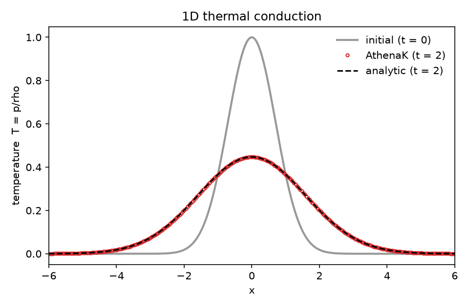
The figure is produced with the bundled reader vis/python/bin_convert.py (run from vis/python/ or with it on your PYTHONPATH):

import numpy as np
import matplotlib.pyplot as plt
from bin_convert import read_binary_as_athdf as read

gamma, amp, D = 5.0/3.0, 1.0, 0.5
def gauss(x, t, n):            # exact n-D Gaussian-pulse solution
    s = 1.0 + 4.0*D*t
    return amp/s**(0.5*n) * np.exp(-x**2/s)

d0 = read("run/bin/heat1d.hydro_w.00000.bin")   # t = 0
d1 = read("run/bin/heat1d.hydro_w.00001.bin")   # t = 2
x = d1["x1v"]
T0 = ((gamma-1)*d0["eint"]/d0["dens"])[0, 0, :]
T1 = ((gamma-1)*d1["eint"]/d1["dens"])[0, 0, :]

plt.plot(x, T0, color="0.6", lw=2, label="initial (t = 0)")
plt.plot(x, T1, "o", ms=3, mfc="none", label="AthenaK (t = 2)")
plt.plot(x, gauss(x, d1["Time"], 1), "k--", label="analytic")
plt.xlabel("x"); plt.ylabel("T = p/rho"); plt.legend(); plt.savefig("heat.png", dpi=150)

2D viscosity

For viscosity, spread the pulse over the x1–x2 plane and carry it in the out-of-plane velocity vz (vel_comp = 3). Because vz does not vary along z, the flow is divergence-free and the pulse obeys the pure diffusion equation with \(D = \nu_{\rm iso}\):

<mesh>
nx1 = 128
nx2 = 128        # a genuinely 2D mesh on [-6,6] x [-6,6]

<hydro>
nu_iso           = 0.5        # D = nu_iso = 0.5

<problem>
viscosity_test   = true
spread_x1        = true
spread_x2        = true       # 2D pulse in the x1-x2 plane
vel_comp         = 3          # diffuse vz (out-of-plane, div(v)=0)
amp              = 1.0

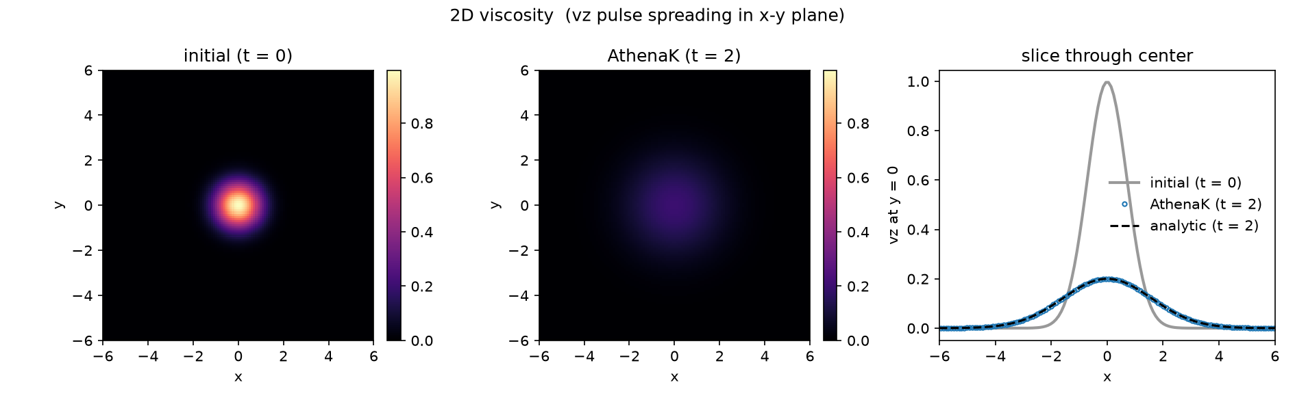
The initial and evolved vz, plus a slice through the center compared with the analytic \(n = 2\) Gaussian:

3D resistivity

Ohmic resistivity uses tst/inputs/diffusion_mhd.athinput. Here the mesh is 3D but the pulse lives in the out-of-plane field component Bz (vel_comp = 3) and spreads in the x1–x2 plane, so it is uniform along z and keeps \(\nabla\!\cdot\!\boldsymbol{B} = 0\). The field then diffuses with \(D = \eta_{\rm O}\):

<mesh>
nx1 = 128
nx2 = 128
nx3 = 16         # 3D mesh; pulse is uniform along x3

<mhd>
eta_ohm          = 0.5        # D = eta_ohm = 0.5

<problem>
resistivity_test = true
spread_x1        = true
spread_x2        = true       # 2D pulse in the x1-x2 plane
spread_x3        = false
vel_comp         = 3          # diffuse Bz
amp              = 1.0

./build/src/athena -i tst/inputs/diffusion_mhd.athinput -d run

A mid-plane slice of Bz (bcc3) matches the analytic 2D Gaussian:

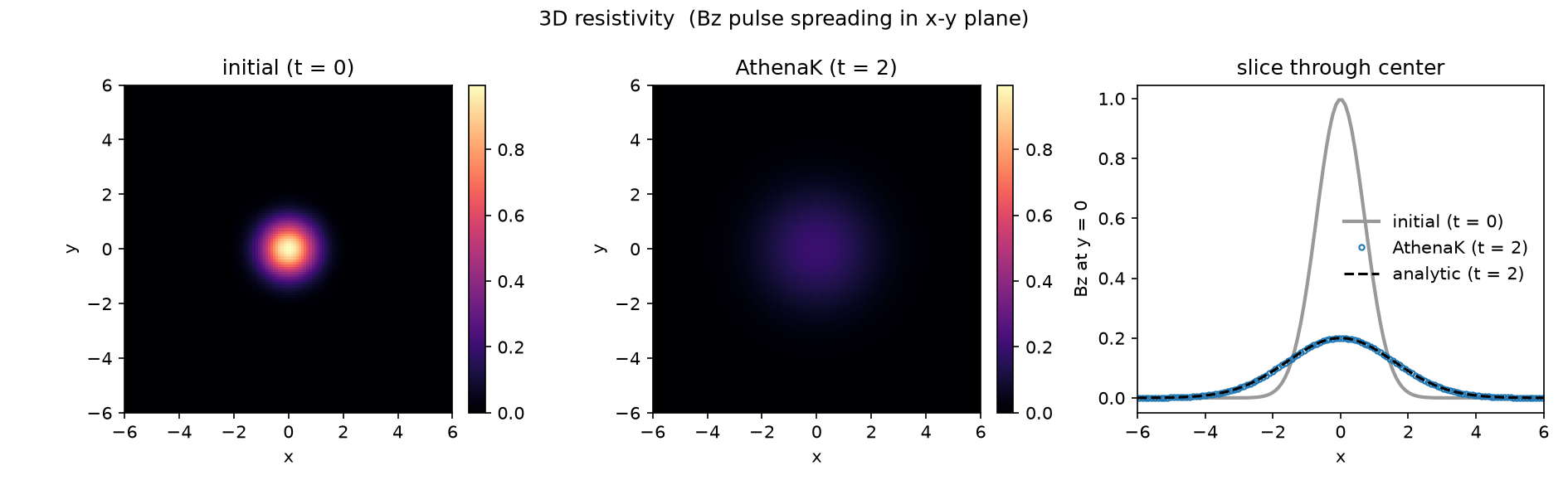
The viscosity and resistivity figures are made just like the conduction one above: read the t = 0 and t = 2 dumps, take the mid-plane slice of velz / bcc3, and overlay the same gauss(x, t, n=2) profile.