Quickstart: Run a Sod Shock Tube
This tutorial walks you through a complete first run of AthenaK from scratch: compiling the code, running a simple built-in test problem, and visualizing the result. The example used here is Sod’s shock tube, a classic 1D hydrodynamics test that runs in seconds on a laptop.
If you have not yet obtained the source, see Download first (a recursive clone that includes the Kokkos submodule is required).
Step 1: Compile
From the top-level repository directory, configure and build a standard CPU executable:
cmake -B build
cmake --build build -j
This produces the executable build/src/athena. (For an optimized release build, GPU
builds, and architecture-specific flags, see Build.)
Step 2: Look at the input file (optional)
While not strictly necessary to run the code, it is helpful to look at the input file
that defines the problem, inputs/hydro/sod.athinput. A few of the key blocks are:
<mesh>
nx1    = 256      # 256 zones...
x1min  = -0.5     # ...spanning x in [-0.5, 0.5]
x1max  = 0.5

<time>
integrator = rk2   # 2nd-order Runge-Kutta
cfl_number = 0.8
tlim       = 0.25  # stop at t = 0.25

<hydro>
eos         = ideal
reconstruct = plm   # piecewise-linear reconstruction
rsolver     = llf   # local Lax-Friedrichs Riemann solver
gamma       = 1.4

<problem>
dl = 1.0   pl = 1.0    # left state:  density 1.0, pressure 1.0
dr = 0.125 pr = 0.1    # right state: density 0.125, pressure 0.1

<output1>
file_type = tab        # 1D tabular output
variable  = hydro_w    # primitive variables
dt        = 0.01       # write every 0.01 in time
See The Input File for the full list of blocks and parameters.
Step 3: Run the simulation
Run the executable, pointing it at the input file:
./build/src/athena -i inputs/hydro/sod.athinput
AthenaK prints cycle/time diagnostics to the screen and, by default, writes outputs
into the current directory. The tab outputs land in a tab/ subdirectory as
Sod.hydro_w.00000.tab through Sod.hydro_w.00025.tab (26 snapshots, one every
dt = 0.01 up to tlim = 0.25), and the history file appears under hst/.
Step 4: Visualize the result
AthenaK ships with lightweight plotting scripts in vis/python. The plot_tab.py
script reads 1D .tab data and can step through the snapshots as an animation:
python3 vis/python/plot_tab.py -i tab/Sod.hydro_w.00000.tab -v dens -n 26
Here -v dens selects the density column and -n 26 reads all 26 frames. The
final frame, at t = 0.25, should look like this:
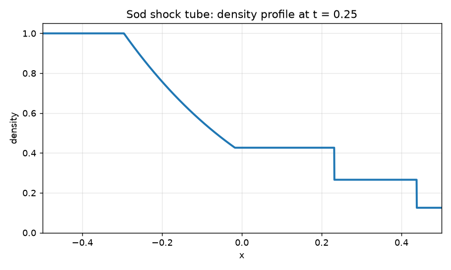
Density profile for Sod’s shock tube at t = 0.25. From left to right you can
see the rarefaction fan, the contact discontinuity (near x = 0.23), and the
shock (near x = 0.44).
See Analysis for more tools, including plot_slice.py for 2D/3D .bin
data and conversion utilities for external visualization software.
Next steps
Try a multidimensional problem, such as
inputs/hydro/blast_hydro.athinputorinputs/hydro/kh2d-sin.athinput, and visualize the.binoutput withvis/python/plot_slice.py.Override parameters on the command line, e.g. increase the resolution with
mesh/nx1=512or change the Riemann solver withhydro/rsolver=hllc.Read Running AthenaK for the full reference on running the code, outputs, and analysis.