Hydrodynamics
Introduction
The hydrodynamics solver is the core fluid module of AthenaK. It integrates the equations of
compressible gas dynamics on the block-based mesh using a high-order Godunov (finite-volume)
scheme: primitive variables are reconstructed to cell faces, an approximate Riemann solver
computes the interface fluxes, and the conserved variables are advanced with a Runge–Kutta
integrator. The solver supports Newtonian, special relativistic, and general relativistic
regimes; which one is used is determined by the coordinate system (see the <coord> block)
and the equation of state.
Hydrodynamics is enabled simply by including a <hydro> block in the input file. For the
magnetized case see Magnetohydrodynamics.
Note
A single run may not contain both <hydro> and <mhd> unless it is a two-fluid
ion–neutral calculation (see Ion-Neutral Fluids).
Inputs
Core options in <hydro>:
eos(mandatory): equation of state,idealorisothermal(isothermal is Newtonian only).gamma(mandatory ifeos = ideal): ratio of specific heats \(\gamma\).iso_sound_speed(mandatory ifeos = isothermal): isothermal sound speed.reconstruct(defaultplm): spatial reconstruction. Options:dc(donor cell),plm(piecewise linear),ppm4andppmx(piecewise parabolic),wenoz(WENO-Z). The higher-order methods require more ghost zones (set<mesh>/nghostto at least 3, or 4 when combined withfofc).rsolver(mandatory): approximate Riemann solver. Valid choices depend on the regime:Newtonian:
llf,hlle,hllc(ideal only),roespecial/general relativistic:
llf,hlle,hllc(SR only)kinematic evolution (
<time>/evolution = kinematic):advect
nscalars(default0): number of passively advected scalars carried by the fluid.fofc(defaultfalse): enable first-order flux correction, which locally falls back to a diffusive first-order update in troubled cells to preserve positivity.
Floors and ceilings (applied during the conserved-to-primitive inversion):
dfloor,pfloor,tfloor,sfloor: density, pressure, temperature, and entropy floors.gamma_max(SR/GR): Lorentz-factor ceiling.
If present, viscosity and conductivity enable explicit dissipation (see
Explicit Diffusion). Gravity, cooling, and other source terms live in a separate
<hydro_srcterms> block (see Source Terms).
Outputs
Request one of the following in an <output>/variable line (see Outputs for output
file types):
hydro_w: all primitive variables (density, velocity, and — for an ideal EOS — internal energy, plus any scalars).hydro_u: all conserved variables (density, momentum, total energy).
Individual components can also be requested (e.g. hydro_w_d for density, hydro_w_vx
for the x-velocity), along with derived diagnostics such as vorticity (hydro_wz,
hydro_w2).
Example: the Liska–Wendroff implosion
The 2D implosion test starts a low-pressure diamond in the corner of a reflecting box; the
converging shocks launch a narrow jet along the diagonal, making it a sensitive test of the
solver’s symmetry and low-diffusion properties. AthenaK ships an input file at
inputs/hydro/lw_implode.athinput using the built-in implode problem generator.
1. Build (the implode generator is built in, so the default build suffices):
cmake -B build
cmake --build build -j
2. Slightly modify the input file. Starting from inputs/hydro/lw_implode.athinput,
sharpen the scheme and switch the output to the native binary format. Set
reconstruct = ppm4 (which needs <mesh>/nghost = 3) and edit the field output block:
<hydro>
eos         = ideal
reconstruct = ppm4      # was plm; needs nghost = 3
rsolver     = hllc
gamma       = 1.4

<output2>
file_type  = bin        # native binary dump
variable   = hydro_w
dt         = 0.05
3. Run and visualize:
./build/src/athena -i inputs/hydro/lw_implode.athinput -d run
python3 vis/python/plot_slice.py run/bin/Implode.hydro_w.00050.bin dens imp_dens.png --notex
The density at late time shows the converging shocks and the thin diagonal jet with its Kelvin–Helmholtz roll-ups:
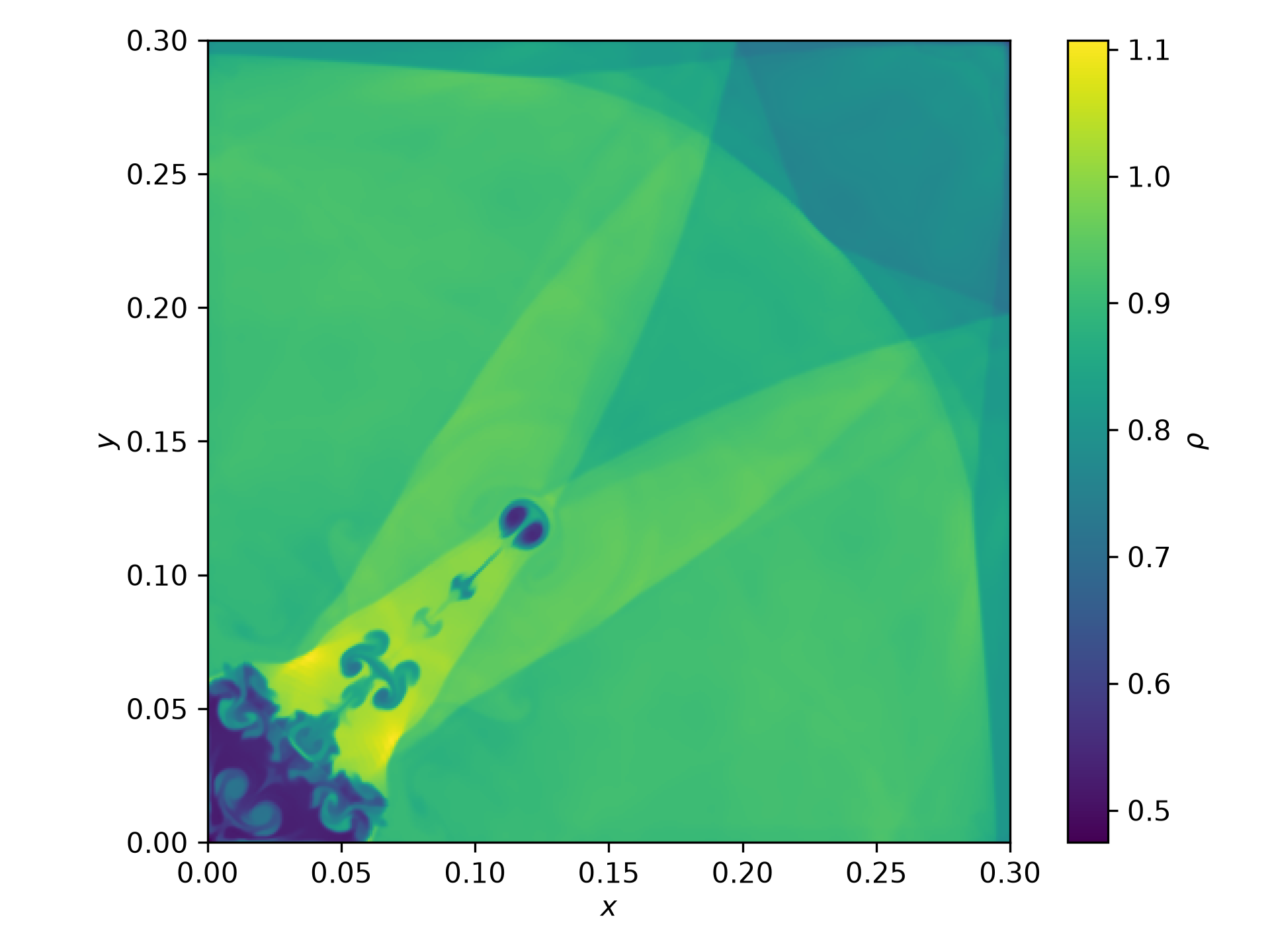
Compare reconstruct = plm with ppm4 or wenoz to see how much the jet and the
small-scale roll-ups depend on the reconstruction order.